University of Pennsyvania
Department of Electrical Engineering
USING MATLAB FOR ELECTRICAL CIRCUITS
1. PLOTTING FUNCTIONS
MATLAB allows you to create plots of functions easily. We will demonstrate
this by the following example.
Suppose we want to plot the folowing three functions:
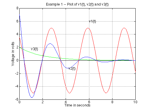
v1(t)=5cos(2t+45 deg.)
v2(t)=2exp(-t/2)
v3(t)=10exp(-t/2)cos(2t+45 deg.)
Further more we want to use red for v1, green for v2 and blue for v3.
In addition we want to label the figure, the horizontal and the vertical
axes as well as each on of the the curves. The following is a sequence
of MATLAB commands that will allow us to do this. This is not a unique
set of commands.
>> t=0:0.1:10;
% t is the time varying from 0 to 10 in steps of 0.1s
>> v1=5*cos(2*t+0.7854);
>> taxis=0.000000001*t;
>> plot(t,taxis,'w',t,v1,'r')
>> grid
>> hold on
>> v2=2*exp(-t/2);
>> plot (t,v2,'g')
>> v3=10*exp(-t/2).*cos(2*t+0.7854);
>> plot (t,v3,'b')
>> title('Example 1 -- Plot of v1(t),
v2(t) and v3(t)')
>> xlabel ('Time in seconds')
>> ylabel ('Voltage in volts')
>> text (6,6,'v1(t)')
>> text (4.25,-1.25,'v2(t)')
>> text (1,1.75,'v3(t)')
Please note the following important point:
1. ; at the end of a line defines the command but does not immediately
execute it.
2. The symbol * is used to multiply two numbers or a number and a function.
3. The combination of symbols .* is used to multiply two functions.
4. The command "hold on" keeps the existing graph and adds the next
one to it. The command "hold off" undoes the effect of "hold on".
5. In the command "text", the first two numbers give the X and Y coordinate
of where the test willo appear in the figure.
6. The command "plot" can plot more than one function simultaneously.
In fact, in this example we could get away with only one plot command.
7. Comments can be included after the % symbol.
8. In the plot command, one can specify the color of the line as well as the symbol: 'b' stands for blue, 'g' for green, 'r' for red, 'y' for yellow, 'k' for black; 'o' for circle, 'x' for x-mark, '+' for plus, etc. For more information type help plot in matlab.
The plot is shown below:
2. COMPLEX NUMBERS
Working with complex numbers in MATLAB is easy. MATLAB works with the
rectangular representation. To enter a complex number, type at the prompt:
EDU>>z = a +bj or a + bi.
example: z = 5-3j
To find the magnitude and angle of z, use the abs() and angle
() function.
Mag = abs(z) Angle = angle(z)
The angle function gives the angle in radians. To convert to degrees
you can use:
angle_deg = angle(z)*180/pi.
Example: V = 
type in MATLAB: V = (5+9j)*(7+j)/(3-2j)
To find the real and imaginary part of a complex number z, type:
real_z=real(z) imag_z=imag(z)
3. SOLVING LINEAR EQUATIONS AND MATRICES
Assume you have the following two linear comples equations with unknown
I1 and I2:
This can be written in matrix form: A.I = B. To solve this in MATLAB one
can use the matrix left division operator:
Or one can also use the following command: I = inv(A)*B
The MATLAB code is as follows:
EDU»A=[600+1250j 100j;100j 60-150j];
EDU»B=[25;0];
EDU»I=A\B
I =
0.0074 - 0.0156i
0.0007 - 0.0107i
EDU»MAGN=abs(I)
MAGN =
0.0173
0.0107
EDU»ANGLE=angle(I)*180/pi
ANGLE =
-64.5230
-86.3244
One uses the abs() operator to find the magnitude of the complex number and the
angle() operator to find the angle (in radians). To get the result in degree we
have multiplied the angle by 180/pi as shown above.
4. FINDING THE ROOTS of a POLYNOMIAL
To find the roots of a polynomial of the form

Define the polynomial as follows: A
= [ am am-1 am-2 ... a1 a0];
The command to for finding the roots is:
roots(A)
As an example consider the following function:

In Matlab:
>> A=[4 12 1];
>> roots(A)
ans =
-2.9142
-0.0858
This works also for complex roots. As an example consider the function:

in Matlab:
>> A=[5 3 2];
>> roots(A)
ans =
-0.3000 + 0.5568i
-0.3000 - 0.5568i
5. FINDING THE POLYNOMIAL WHEN THE ROOS ARE KNOWN
Suppose that you have the following expression F(s) and would like to find the coefficient of the corresponding polynomial:

This is defined in Matlab by a column vector of the roots:
roots = [a1; a2; a3 ];
One finds than the coefficient of the polynomial, using the "poly" command:
poly(roots);
As example consider the function F(s) = s(s+50)(s+250)(s+1000). To find the coefficient of the coresonding polynomials, one first define the column vector of the roots:
roots=[0; -50; -250; -1000 ];
The coefficients are then found from the poly command:
coeff = poly(roots)
which will give:
coeff = 1 1300 312500 12500000 0
corresponding to the polynomial,

6. TRANSFER FUNCTIONS H(s) and BODE PLOT
6a. Using the Bode command when the transfer function is specified as a ratio of two polynomials.

with m < n
in MATLAB, specify D and N:
num = [am am-1 ... a1
ao] den = [bn bn-1 ... b1 bo]
to plot the transfer function (magnitude and phase), type:
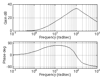
Example: H(s) = (0.5s +1)/(1E-4s2 + 0.01s +1)
In Matlab:
num = [0.5 1];
den = [1e-4 0.01 1] ;
bode (num, den)
One can also specify the frequency axis w (radial frequency):
For the same example one can specify the frequency range as a vector:
w = [0.1: 0.1: 10000];
bode(num,den,w)
grid on
in which w is the frequency. The resulting graph is shown below.

6b. Plotting a transfer function when Poles and Zeros are given:
Often, the transfer function is specified as a function of its poles
and zeros, in the form:
H(s)=K(s+s1)(s+s2)(1+as + bs2)/ (s+s3)(s+s4)(1+cs + ds2).
In that case one can find the polynomial of the nominator and denomator
first by using the
poly function and the conv function. One first defines
a column vector of the roots (-s1, -s2, etc.):
root_num=[-s1; -s2; ...];
To find the polynomial corresponding to these roots, use
If necessary one can multiply the d1 polynomial with the quadratic term
using the
conv function. First define the polynomial
corresponding to the quadratic term:
d2=[b a 1];
num=conv(d1,d2)
The same can be done for the denominator.
Example:
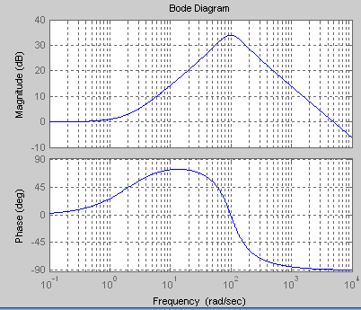
H(s)=72x(s+2)/s(s+50)(s+250)(s+1000)(s2 + 2.4s + 144)
First find the coefficent of the polynomial corresonding to s(s+50)(s+250)(s+1000) of the denominator:
rootsd1=[0; -50; -250; -1000 ];
d1=poly(rootsd1);
Then, one multiply this polynomial with the remaining quadratic term (s2 + 2.4s + 144) in the denominator (d2 defines the quadratic term):
d2=[1 2.4 144];
In which "den" corresponds to the polynomial of the denominator. Finally, one can plot the Bode Diagram:
An altnerative command to plot the magnitude and phase of a transfer function
is:
freqs(num, den)
6c. Using the plot command when the transfer function is not specifed as a ratio of polynomials
The previous transfer function
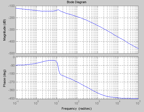
H(s) = 72x(s+2)/s(s+50)(s+250)(s+1000)(s2 + 2.4s + 144)
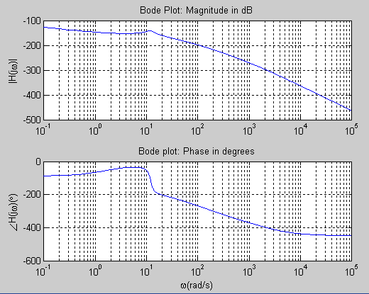
in which s=jw, can be plotted using the plot function in Matlab.We need to define the range of the indpendent variable w before plotting the fucntion H(jw).
>> w=[0.1: 0.1: 10^5];
>> H=72*(2+j*w)./(j*w.*(50+j*w).*(250+j*w).*(2000+j*w).*(144+2.4*j*w+(j*w).^2));subplot(2,1,1);
>> subplot(2,1,1);
>> semilogx(w,20*log10(abs(H)));
>> grid on
>> ylabel('|H(j\omega)|');
>> title('Bode Plot: Magnitude in dB');
>> subplot(2,1,2);
>> semilogx(w,unwrap(angle(H))*180/pi);
>> grid on;
>> xlabel('\omega(rad/s)');
>> ylabel('\angleH(j\omega)(\circ)');
>> title('Bode plot: Phase in degrees');
Notice:
- When defining the tranfer function H, the . operator needs to be use in order to perform array mathematics on an element-by-element basis.
- The subplot(n,m,p) instructs matlab that there will be n by m plots and to select the pth plot. In our case subplot(2,1,1) indicates that we want to have two plots on to of each other, and that we have selected the 1st one (top one) as the current one.
- The function semilogx is similar to the plot function except that a logarithmic scale (base 10) is used for the x axis. We are plotting the log (base 10) of the magnitude (abs) of the function H.
- Next we want to plat the angle. This is done by first specifying the position of the plat: subplot(2,1,2).
- Then, we instruct matlab to plot the angle, using the semilogx command. Since the angle() command gives the angle in radians, we multiply it by 180.pi to get the phase in degrees. The unwrap is included to ensure that the phonse does jump from +180 t o-180 degrees.
The results is shown below. As can be seen it is the same graph as the one obtained from the Bode command.

7. OUTPUT of a SYSTEM DEFINED BY A TRANSFER FUNCTION
7.a Response to any input x(t)
Assume that the system is described by a transfer function H(s)=NUM(s)/DEN(s) where NUM and DEN contain the polynomial coefficients in descending powers of s.
One can then plot the output of the system for a given input signal x(t). As an example, lets consider a simple 2nd order low pass filter with a cutoff frequency of 100 rad/s:

in which NUM = [0 1] and DEN = [10^-4 0.02 1].
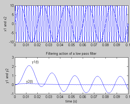
Lets apply two sinusoidial input signals x1 and x2 of frequency 50 Hz:and 500 Hz, respectively. The the corresonding output sigals are called y1 and y2, respectively. Since the system filters out higher frequencies we expect that the output y2 is considerably smaller than y1. We can plot the outputs of y1 and y2 using the lsim comment:
LSIM(NUM,DEN,U,T) command.
in which U is the input and T is the time. The matlab code for the filter and the input and output signals is as follows.
>> t=0:0.0001:0.1;
>> x1=10*sin(2*pi*50*t);
>> x2=10*sin(2*pi*500*t);
>> y2=lsim(NUM,DEN,x2,t);
>> y1=lsim(NUM,DEN,x1,t);
>> subplot(2,1,1);
>> plot(t,x1);
>> hold on
>> plot(t,x2);
>> subplot(2,1,2);
>> plot(t,y1);
>> hold on
>> plot(t,y2) ;
>> text(0.015, 2.5, 'y1(t)');
>> text(0.01, 0.35, 'y2(t)');
>> title('Filtering action of a low pass filter');
>> ylabel('y1 and y2');
>> xlabel('time (s)');
>> subplot(2,1,1);
>> ylabel('x1 and x2') ;
The graphs of the inputs x1 and x2 (top graph) and the outputs y1 and y2 (bottom graph) illustrates the effect of the filtering action.

7.b Step Response
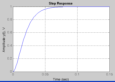
Again, assume that the system is described by a transfer function H(s)=NUM(s)/DEN(s) where NUM and DEN contain the polynomial coefficients in descending powers of s. The step response y(t) of the system with the above transfer function is obtained by the command step.
Step(NUM,DEN
Again An example, lets plot the step response to the 2nd order low-pass filter used above,

in which NUM = [0 1] and DEN = [10^-4 0.02 1].
>> num=[0 1];
>> den=[10^-4 0.02 1];
>> step(num,den)

Go to
ESE215, ESE216
Created by J. Van der Spiegel <jan@ee.upenn.edu>;
Feb. 11, 1997;
Updated by J. Van der Spiegel, March 17, 2009.
