Homework 2 - CIS501 Fall 2010
| Instructor: | Prof. Milo Martin |
|---|---|
| Due: | Thursday, 21st (at the start of class) |
| Instructions: | Your solutions to this assignment must either be hand-written clearly and legibly or, preferably, typed. Show all your work to document how you came up with your answers. |
Cost and Yield. We talked about cost and yield issues only briefly in class, so this question will introduce you to the cost issues in manufacturing a design.
Your company's fabrication facility manufactures wafers at a cost of $50,000 per wafer. The wafers are 300mm in diameter (approximately 12 inches). This facility's average defect rate when producing these wafers is 1 defect per 500 mm2 (0.002 defects per mm2). In this question, you will calculate the manufacturing cost per chip for 100 mm2, 200 mm2, and 400 mm2 chips.
The first step is to calculate the yield, the percentage of chips manufactured that are free of manufacturing defects using the following yield equation (from the appendix of the Patterson and Hennessy textbook):
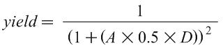
Where A is the area of the chip in mm2, D is the defects per mm2, and yield is a number between 0 and 1. Intuitively, this equation shows that if either the area of the chip or the defect rate increases, the yield decreases.
Based on this yield equation, what is this facility's yield for chips of 100 mm2, 200 mm2, 400 mm2?
Approximately how many good (defect-free) chips can be made from each wafer for each of these three chip sizes? (You can ignore the "square-peg-in-round-hole" effect.)
What is the manufacturing cost for each of these three chip sizes?
Performance I. Computer A executes the ARM ISA and has a 2.5Ghz clock frequency. Computer B executes the x86 and has a 3Ghz clock frequency. On average, programs execute 1.5 times as many ARM instructions than x86 instructions.
- For Program P1, Computer A has a CPI of 2 and Computer B has a CPI of 3. Which computer is faster for P1? What is the speedup?
- For Program P2, Computer A has a CPI of 1 and Computer B has a CPI of 2. Which computer is faster for P2? What is the speedup?
Performance II. Assume a typical program has the following instruction type breakdown:
- 30% loads
- 10% stores
- 50% adds
- 8% multiplies
- 2% divides
Assume the current-generation processor has the following instruction latencies:
- loads: 4 cycles
- stores: 4 cycles
- adds: 2 cycles
- multiplies: 16 cycles
- divides: 50 cycles
If for the next-generation design you could pick one type of instruction to make twice as fast (half the latency), which instruction type would you pick? Why?
Averaging. Assume that a program executes one branch ever 4 instructions for the first 1M instructions and a branch every 8 instructions for the next 2M instructions. What is the average number instructions per branch for the entire program?
ISA Modification and Performance Metrics. You are the architect of a new line of processors, and you have the choice to add new instructions to the ISA if you wish. You consider adding a fused multiply/add instruction to the ISA (which is helpful in many signal processing and image processing applications). The advantage of this new instruction is that it can reduce the overall number of instructions in the program (converting some pairs of instructions into a single instruction). The disadvantage is that its implementation requires extending the clock period by 10% and increases the CPI by 15%.
Calculate under what conditions would adding this instruction lead to an overall performance increase.
What qualitative impact would this modification have on the overall MIPS (millions of instructions per second) of the processor?
What does this say about using MIPS as a performance metric?
Amdahl's Law. A program has 10% divide instructions. All non-divide instructions take one cycle. All divide instructions take 20 cycles.
- What is the CPI of this program on this processor?
- What percent of time is spent just doing divides?
- What would the speedup be if we sped up divide by 2x?
- What would the speedup be if we sped up divide by 5x?
- What would the speedup be if we sped up divide by 20x?
- What would the speedup be if divide instructions were infinitely fast (zero cycles)?
Caching. Consider the following progression of on-chip caches for three generations of chips (loosely modeled after the Alpha 21064, 21164, and 21264).
Assume the first generation chip had a direct-mapped 8KB single-cycle first-level data cache. Assume Thit for this cache is one cycle, Tmiss is 100 cycles (to accesses off-chip memory), and the miss rate is 20%. What is the average memory access latency?
The second generation chip used the same direct-mapped 8KB single-cycle first-level data cache, but added a 96KB second-level cache on the chip. Assume the second-level cache has a 10-cycle hit latency. If an access misses in the second-level cache, it takes an additional 100 cycles to fetch the block from the off-chip memory. The second-level cache has a global miss rate of 4% of memory operations (which corresponds to a local miss rate of 20%). What is the average memory access latency?
The third generation chip replaced the two-levels of on-chip caches with a single-level of cache: a set-associative 64KB cache. Assume this cache has a 5% miss rate and the same 100 cycle miss latency as above. Under what conditions does this new cache configuration have an average memory latency lower than the second generation configuration?
Effectiveness of Compiler Optimizations. The compiler's goal is to generate the fastest code for the given input program. The programmer specifies the "optimization" level the compiler performs. To ask the compiler to perform no compiler optimizations, the "-O0" flag can be used (that is "dash oh zero"). This is useful when debugging. It is also the fastest compilation and the least likely to encounter bugs in the compiler. The flag "-O2" (dash oh two) flag enables optimizations, the "-O3" (dash oh three) enables even more optimizations. Finally, the flag "-funroll-loops" enables yet another compiler optimization.
This question asks you to explore the impact of compiler optimizations using the following simple single-precision "a*x+y" (saxpy) vector-vector operation:
#define ARRAY_SIZE 1024

float x[ARRAY_SIZE];
float y[ARRAY_SIZE];
float z[ARRAY_SIZE];
float a;

void saxpy()
{
  for(int i = 0; i < ARRAY_SIZE; i++) {
    z[i] = a*x[i] + y[i];
  }
}
See code.c for this code with all the proper defines. Log into minus.seas.upenn.edu via SSH, and compile the code with three different levels of optimization:
gcc -O0 -Wall -std=c99 -S code.c -o code-O0.s
gcc -O2 -Wall -std=c99 -S code.c -o code-O2.s
gcc -O3 -Wall -std=c99 -S code.c -o code-O3.s
gcc -O3 -funroll-loops -O3 -Wall -std=c99 -S code.c -o code-O3-unrolled.s
This will create four .s files in the directory (code-O0.s, code-O2.s, code-O3.s, and code-O3-unrolled.s). These files are the x86 assembly of this function. You can ignore everything except the code between the label saxpy and the return statement (ret).
Note
You don't have to understand much x86 code to answer the following questions, but you may find seeing actual x86 code interesting. For example, instead of using "load" and "store" instructions, in x86 these instructions are both "mov" (move) instructions. An instruction like add %ecx, (%esp) performs both a memory access and an add (an example of a CISC-y x86 instruction). The x86 ISA also has some more advanced memory addressing modes, such Also, x86 uses condition codes, so jump (branch) instructions don't have explicit register inputs. If you want to lookup an x86 instruction, you may find the Intel x86 reference manual useful: http://www.intel.com/products/processor/manuals/
For each of these files, answer the following questions:
- What is the static instruction count (the number of instructions in the source code listing) of the loop (just ignore the header and footer code to count the number of instructions in the loop)?
Based on the number of instructions in the loop (above) and the number of iterations of the loop in each .s file, calculate the approximate number of dynamic instructions executed by the loop in the function (approximately, to the nearest few hundred instructions).
Assuming a processor with a CPI of 1, how much "faster than" is the -O2 than -O0? How much faster is -O3 than -O2? How much is unrolled faster than -O3?
- When comparing the last two optimized .s files, how does the number of static instructions relate to the dynamic instruction count? Give a brief explanation.
- Using what you learned from this data, what is one advantage and one disadvantage of loop unrolling?
Next, run the four versions. To do this, link each source file with driver.c and run it. The driver calls the function 1 million (1,000,000) times and reports the runtime in seconds:
gcc -static code-O0.s driver.c -o code-O0
gcc -static code-O2.s driver.c -o code-O2
gcc -static code-O3.s driver.c -o code-O3
gcc -static code-O3-unrolled.s driver.c -o code-O3-unrolled

./code-O0
./code-O2
./code-O3
./code-O3-unrolled
Note
You may be surprised by the large difference in performance between -O2 and -O3. In this version of GCC, enabling -O3 also enables automatic vectorization. This computation is one that GCC can vectorize, so GCC uses "packed" versions of the various instructions that operate on four elements of the array at a time (that is, load four values, multiple four value, store four values, etc.).
- Give the runtime of each of these versions. How much faster is -O2 that -O0? How much faster is -O2 over -O3? How much faster is unrolled over -O3? How does this compare to your estimate above based only on instruction counts?
The clock frequency of the processors in "minus.seas.upenn.edu" is 3.0 Ghz (3 billion cycles per second). Based on your estimate of the number of instructions in each call to the function and that driver.c calls the function 1 million times, calculate the CPI of the processor running each of these programs.
What do the above CPI numbers tell you about these compiler optimizations? You may wish to calculate the IPC of each, as sometimes it is easier to reason about IPC (instructions per cycle) rather than CPI (the inverse metric).
Pipelining and Load Latency. In the five-stage pipeline discussed in class, loads have one cycle of additional latency in the worst case. However, if the following instruction is independent of the load, the subsequent instruction can fill the slot, eliminating the penalty. Using the trace format used in the first assignment (see Trace Format document), this questions asks you to simulate different load latencies and plot the impact on CPI.
Based on the frequency of loads for the trace you calculated in the first assignment, calculate the CPI (cycles per micro-instruction) using the simple non-pipelined model in which all non-load instructions take one cycle and loads take n cycles. What is the CPI if loads are two cycles (one cycle load-use penalty)? What about three cycles (two cycle load-use penalty)?
Plot the CPI (y-axis) as the load latency (x-axis) varies from one to 15 cycles (the line should be a straight line).
Using the simulation described below, add a second line to the graph described above, but use the CPI calculated by the simulations.
When the load latency is two cycles, what is the performance benefit of allowing independent instructions to execute versus not? (Express your answer as a percent speedup.) What about with three cycles?
What to turn in: Turn in the graph (properly labeled) and the answers to the questions above.
Simulation description. Instead of simulating a specific pipeline in great detail, we are going to simulate an approximate model of a pipeline, but with enough detail to capture the essence of the pipeline. For starters, we are going to assume: full bypassing (no stalls for single-cycle operations), perfect branch prediction (no penalty for branches), no structural hazards for writeback register ports, and only loads will have latency of greater than one. Thus, the only stall in the pipeline is load-use stalls of dependent instructions. As loads never set the flags (condition codes), you can also ignore those.
There are several ways to simulate such a pipeline. One way is to model the pipeline using a "scoreboard". The idea is that every register has an integer associated with it (say, an array of integers). This value represents how many cycles until that value is "ready" to be read by a subsequent instruction. Every cycles of execution decrement these register values, and when a register reaches zero, it is "ready". If any of an instruction's input registers are not ready (a value greater than zero indicates it isn't ready), that instruction must stall. Whenever an instruction writes a value, it sets its entry in the scoreboard of its destination register (if any) to the latency of the instruction.
Valid register values. Recall that any register specified as "-1" means that it isn't a valid source or destination register. So, if the register source or destination is -1, you should ignore it (the input is "ready" and the output register doesn't update the scoreboard). You may assume the register specifiers in the trace format are 50 or less.
Algorithm. The suggested simulation loop is:
next_instruction = true
while (true):
  if (next_instruction):
    read next micro-op from trace
    next_instruction = false

  if instruction is "ready" based on scoreboard entries for valid register inputs:
    if the instruction writes a register:
      "execute" the instruction by recording when its register will be ready
    next_instruction = true

  advance by one cycle by decrementing non-zero entries in the scoreboard
  increment total cycles counter
The above algorithm captures the basic idea. Notice that if an instruction can't execute, nothing happens. Thus, no new instruction is fetched the next cycle. However, all of the ready counts have been decremented. Thus, after enough cycles have past, the instruction will eventually become ready.
Note
As a simplification, you can also ignore out-of-order writes to destination registers (that is, stalling to ensure that slower load doesn't overwrite the register that was already written by a subsequent faster instruction). I modeled it in my simulator, and it just doesn't make a difference in this case.
To help you debug your code, we've provided some annotated output traces of the first two hundred lines of the GCC trace file (gcc-200-2-cycle.txt and gcc-200-9-cycle.txt). The format for the output is:
0     1 -1 (Ready)    -1 (Ready)     -> 13  -  -------------1------------------------------------
1     2 -1 (Ready)    -1 (Ready)     -> 13  -  -------------1------------------------------------
2     3 -1 (Ready)     5 (Ready)     -> 45  L  ---------------------------------------------2----
3     4 45 (NotReady)  3 (Ready)     -> 44  -  ---------------------------------------------1----
4     4 45 (Ready)     3 (Ready)     -> 44  -  --------------------------------------------1-----
5     5 -1 (Ready)     5 (Ready)     ->  3  L  ---2----------------------------------------------
6     6 -1 (Ready)    -1 (Ready)     ->  0  -  1--1----------------------------------------------
7     7 -1 (Ready)    -1 (Ready)     ->  0  -  1-------------------------------------------------
8     8 -1 (Ready)    -1 (Ready)     -> 12  -  ------------1-------------------------------------
The columns (left to right) are: cycle count, micro-op count, source register one (ready or not ready), source register two (ready or not ready), the destination register, load/store, and the current contents of the scoreboard (the cycles until ready for that register or "-" if zero).
As can be seen above, the first load causes a stall as it is followed by a dependent instruction (notice that the instruction is repeated, as it stalled the first time). However, the second load is followed by an independent instruction, so no stall occurs.
Addendum
- [Oct 14] - Added '-static' compiler flag. Without this the global variables are oddly aligned, which causes the performance results to be quite odd.
- [Oct 12] - Added pipeline question