Admin
Project 1
- Due Today (3/11)
- Netlist request - "Don't ask, don't tell" policy: You have the option of writing your name on your schematic or not. If you don't, your name will not be given to anyone who might try to find out.
- Talks Thursday
Project 2
- Assignment out today
- Sign up for an appointment w/ Andre'
Partitioning
- "Solves" placement for strict hierarchical interconnect
(e.g. Aggarwal and Lewis, also HP PLASMA)
- Often used to initialize placement
- Balanced partitions NP-complete, in general
- Fast heuristics exist (Fiduccia-Mattheyses)
- Doesn't address critical path delay
Partitioning Problem
- Given: netlist of interconnected cells
- Partition into two (roughly) equal halves (A,B), minimizing the number of nets shared by halves
- "Roughly Equal" Balance Condition:
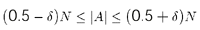
The goal is to discover the bisection cut
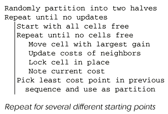
Fiduccia-Mattheyses
(refinement on Kernighan-Lin)
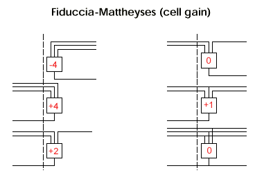
Number in red indicates gain if cell is moved to the other partition.
Fiduccia-Mattheyses (recompute cell gain)
- For each net, keep track of number instances in each partition
- critical net has one element on one side
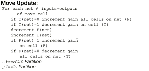
Key thing to note is that each net is considered separately.
Value of (not change to) cell gain (before move):
Gain deltas associated with move:
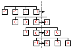
Fiduccia-Mattheyses (data structures)
N
cells
- partition counts A, B
- consumers
- inputs
- locked status
two arrays gain arrays
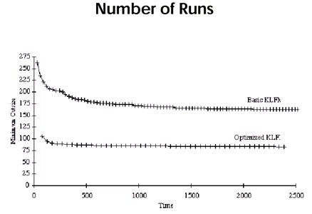
Fiduccia-Mattheyses (Optimization Sequence)
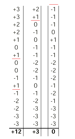
Red line indicates point at which "best" progress is reached. This is the partition chosen for the start of the next iteration. Note that in the first pass, there are two "best" partitions.
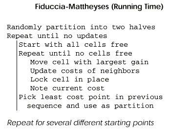
- Claim: small number of passes (constant?) to converge
- Small, constant number of random starts
- N
cell updates
- Updates K + fanout (average fanout K)
- Maintain ordered list O(1) per move
- Running time: O( KN ), assuming that it converges in ~constant time.
Tweaks on Fiduccia-Mattheyses
Tweaks exist to speed up Fiduccia-Mattheyses:
- clustering
- technology mapping
- initial partition
- number runs
- maximum partition size variation

- replication
(Comparisons from Hauck and Boriello '96)
Clustering
1. group together several leaf cells into one larger for FM partitioning
2. run partition on clustered cells
3. uncluster, keep partitions (uncluster iteratively rather than all at once)
4. run partition again (with previous step as initial partition)
Benefits:
- catch local connectivity global algorithm may miss
- runs faster (smaller N)
- FM work better with 6+ input nodes (?)
Connectivity Clustering
- examine nodes in random order
- cluster node with neighbor with highest "connectivity"
- best of several techniques
- 30% better than random clustering
- 16% faster than random clustering
Technology Mapping
Better to partition at "gate" level, than after mapped to LUTs.
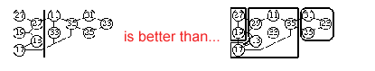
In this example, two wires cut v/s three.
Initial Partition
Random best:
- Random (82.4)
- Seeded (95.3)
- Breadth-First (86.7)
- Depth-First (86.5)
v/s spectral initial:
- Random (68.6)
- spectral (73.5)
Over the long run, random can do better, since w/ spectral initial placement, the placement is identical every time --> no potential for improvement.
Note that most of the gain is attained in the first 400 steps. Beyond that, improvement is incremental.
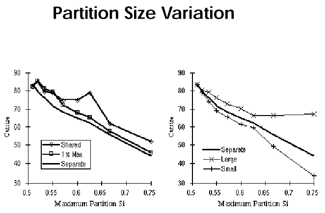
Smaller cut size can be achieved if more variation in partition size is allowed.
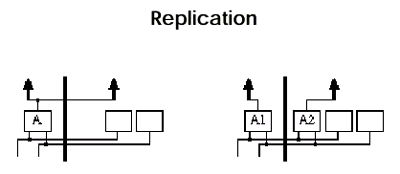
Trade some additional area logic for smaller cut size. (replication data/figures from Enos, Hauck, Sarrafzadeh '97)
On left, cut size is three; on the right, it is two.
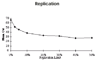
5% additional logic --> 38% smaller cut

Significant gain for relatively little cost in area.
50% --> 50+% smaller
Partition Wrapup
- Hack and Boriello "Optimized"
- Half size of vanilla FM (w/o replication)
- 30-40% better if allow 5% replication.
- All tweaks address partition quality and execution time, not critical path.
- ?are there ways to fold time into this heuristic?
- Look for a bigger hammer: Simulated Annealing
Simulated Annealing
- Analogy to cooling of materials: search for minimum cost
- ~search for minimum energy state in physical system.
- Atoms trying to find minimum energy
- Thermal energy (kT) allows atoms to move - changing configurations within energy state.
- i.e. energy barrier less than kT --> thermal energy allows intermediate fluctuations necessary to move between energy states.
- Random walk - influenced by energy function.
- T
high - lots of energy, atoms free to move around
- T
low - little free energy, atoms localized
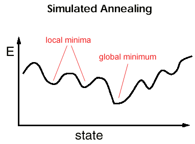
Need to hill climb in order to find the global minimum. Q: how to do this in an n-dimensional space?
- Physical system, we know: if cool too fast, will freeze in defects (high-energy states); won't find structured, low-energy states, only local minima
- must carefully anneal
- lower temperature slowly
- spend considerable time around freezing point so atoms can relocate themselves into minimum energy states before they loose sufficient energy to move
Metropolis Algorithm for simulating collection of atoms:
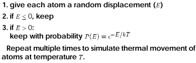
"Good" moves are always kept, "bad" moves are kept with a probability that is a function of the current "temperature". Bad moves are kept in the hope that they will enable hill climbing.
Simulated Annealing
- Melt material (start with high T)
- lower temperature slowly
- stay at each temperature long enough to reach steady state
don't want to cool too quickly, else we "freeze" in high-energy states
- stop when temperature low enough to "freeze"
- no further changes
- Annealing schedule - sequence of temperatures and lengths of time at each temperature
- If cool slowly enough, find state close to minimum energy state.
Optimization Analog
- Energy --> cost function
- Temperature --> freedom to make non-greedy moves. Moves that make your solution worse are sometimes taken.
- Start at high temperature - most any move accepted --> virtually random moves.
- Lower temperature slowly - makes more "greedy"
- At T = 0 reduces to greedy moves only (only good moves are taken)
Using SA
To use:
- Identify moves
- Define cost function - effectiveness of simulated annealing often dependent on how cost function is chosen.
- Power of technique is ~arbitrary cost function. (I.e., you can apply it to most anything.)
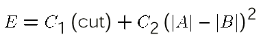
Formulation of Cost Function for Partitioning
Partitioning:
- Move:
swap partitions
- Cost:
cut-set and balance
Formulation for Partitioning and Timing
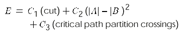
- Easy to add constraints to cost function.
- May be tricky to calculate E efficiently.
(often the limit to complexity/accuracy of E will be evaluating a very large number of potential moves)
Formulation for Placement
Move:
swap location of two cells
Cost:
- total wire length
- channel congestion
- wire delay
May limit distance swaps considered by temperature
Intuition: do global optimization first, later focus on local optimization.
Simulated Annealing Wrapup
- Big-hammer for hard optimization problems
- General cost model - accommodates most any constraints
- If cool slowly enough, will get good results
- Finesse in working out parameters
- Cost should be cheap to update
- Annealing schedule can be tricky to optimize
(balance speed versus quality)
- ...generally takes a long time...
(...why PPR is slow)