**CIS 192 Homework 4: Machine Learning 🤖** **Due Fri March 3, 2023 11:59 pm EST** (#) Learning objectives - Familiarization with 3rd party modules - `scikit-learn` - `matplotlib` - `numpy` - Intuition for machine learning concepts - over/under-fitting and model complexity - feature preprocessing: standardization (#) Starter files - [hw4.py](hw4/hw4.py) - [hw4_utils.py](hw4/hw4_utils.py) !!! tip Make sure to download the `hw4_utils.py` file and place it in the same directory as your `hw4.py` file! (#) Setting up Like HW 3, we will be using third party modules for this homework assignment. Make sure you have NumPy, Scikit-learn, and Matplotlib installed before proceeding with the assignment. 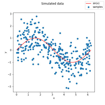~~~~~~ bash $ pip3 install numpy $ pip3 install matplotlib $ pip3 install scikit-learn ~~~~~~ (#) Part 1: Exploring the bias-variance tradeoff As discussed in lecture, a key consideration in building any machine learning model is the bias-variance tradeoff. Without getting into the mathematical details, we have to balance "bias" (which increases when models are too simple) against "variance" (which increases when models are too complex). We will explore this by running a simulated experiment trying to fit polynomials to a sine curve. Pictured below is a sample of the curve we will be trying to fit, a result of calling `generate_data()` in the `hw4_utils.py` starter file we provide:  (##) Controlling complexity using polynomials In this setting, we will control the complexity of our model by the number of polynomial features we provide as arguments to a linear regression: the more polynomial features we provide, the more "complex" our model is. To do this, you will implement the `make_poly_features(X, max_deg)` function. The parameter `X` passed into `make_poly_features` will be the initial one-dimensional array of $X = \{x_1, x_2, \ldots, x_n\}$ values with $n$ samples, and the `max_deg` will be the maximum degree polynomial you will generate. Below are some examples of what this function will output: $$ \text{make_poly_features(X, 2)} = \begin{bmatrix} x_1 & x_1^2 \\ x_2 & x_2^2 \\ \vdots & \vdots \\ x_n & x_n^2 \end{bmatrix}_{(n \times 2)} $$ $$ \text{make_poly_features(X, 3)} = \begin{bmatrix} x_1 & x_1^2 & x_1^3\\ x_2 & x_2^2 & x_2^3\\ \vdots & \vdots & \vdots\\ x_n & x_n^2 & x_n^3 \end{bmatrix}_{(n \times 3)} $$ !!! WARNING For full credit, you should provide a vectorized implementation using broadcasting (no for loops) of `make_poly_features()`. The [NumPy broadcasting tutorial](https://numpy.org/devdocs/user/basics.broadcasting.html) may be a useful review of these concepts. (##) The train/test split To train a machine learning model and to make predictions, we need to first divide our data into mutually exclusive *train* and *test* sets. This is to prevent the model from **overfitting** -- if you test your model on examples it has already seen before, it may produce overly optimistic performance and may not generalize well. Think to the exam example we talked about in class: if you saw the exact same question from a practice exam on the actual exam you're very likely to get the question right, but not necessarily because you learned the concept, but rather you remember the answer from studying. You will implement the method `make_train_test_idxs(X, train_pct)`, which will split your array into two separate arrays: one for training and one for testing. This split will be based on indices of the array. Example usage is below: ~~~~~~~~~~~~~~~~ python >>> X = np.ones((8, 5)) # X has 8 samples, 5 features # the training set should be half of the data >>> train_idx, test_idx = make_train_test_idx(X, train_pct=0.5) >>> train_idx array([6, 2, 1, 7]) >>> test_idx array([3, 0, 5, 4]) # note that no indices are shared # can now split X into training and testing partitions >>> train_X, test_X = X[train_idx], X[test_idx] ~~~~~~~~~~~~~~~~ (##) Fitting a linear regression model We will now leverage the scikit-learn APIs to fit a simple linear regression model to the data. Use your implementation of `make_poly_features` and the [LinearRegression](https://scikit-learn.org/stable/modules/generated/sklearn.linear_model.LinearRegression.html) model to complete the `fit_poly_regression(X, y, deg)` function. 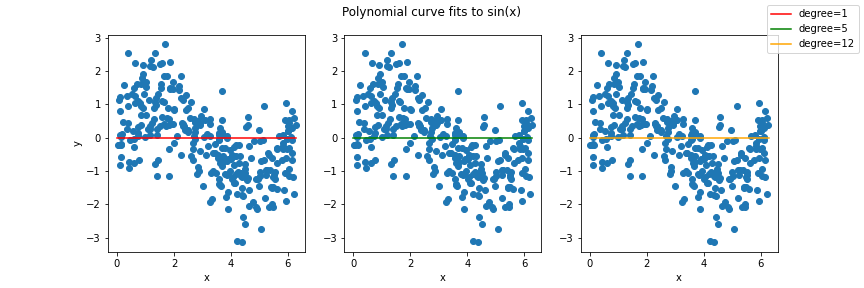(##) Visualizing predicted curves Once you have implemented the `fit_poly_regression()` function, you will then plot learned curves for polynomials of degree {1, 5, 12}, fit to the sine data in the `plot_curves()` function. We have provided starter code in the `__main__` function that you will run after implementing the functions above. 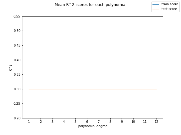Pictured below is the template for the plot styling you need to replicate, with the actual polynomial curves you need to plot replaced with horizontal lines:  (##) Running an experiment In addition to visualizing the complexity of different polynomial degrees, we can quantify how good our predicted curves are through [$R^2$ scores](https://en.wikipedia.org/wiki/Coefficient_of_determination): the higher $R^2$ is, the better our curves fit the data. We have provided a `run_experiment()` function that simulates many datasets and fits models of varying degrees to the data, returning both training $R^2$ and testing $R^2$ scores. Your job is to plot the mean of both these scores as a function of the polynomial degree in `plot_scores()`. We have provided starter code in the `__main__` function that you will run after implementing the functions above. Pictured below is the template for the plot styling you need to replicate, with the actual mean training and test score values you need to plot replaced with horizontal lines:  (##) Discussion questions [1 pt] Once you have completed your implementation of `plot_scores()` and `plot_curves()`, answer these questions **in the multi-line comment** we provide at the bottom of `hw4.py`. 1. In your `poly_curves.png`, which polynomial degree out of {1, 5, 12} matches the true sine curve the best (i.e. neither overfit nor underfit)? 2. In machine learning, the concept of [Occam's Razor](https://en.wikipedia.org/wiki/Occam%27s_razor#Science_and_the_scientific_method) is often a good guideline for choosing models: we want the best test scores, but we prefer a simpler model if the scores are similar. For this problem, this can be seen as the choosing the lowest degree polynomial where the test scores stop increasing. Looking at your `poly_scores.png`, which degree polynomial should we choose to best satisfy the Occam's Razor guideline? (#) Part 2: Training a breast cancer classifier Part 1 examined fitting a model to a sine curve, which is a *regression* task since the output we are trying to predict has continuous values. We can also use machine learning for *classification*, where the output we are trying to predict are discrete labels, such as trying to label a tumor as {malignant, benign}, or trying to label an image of an animal as {dog, cat, bird, fish}. Here we will explore a breast cancer classification dataset to train a machine learning classifier. (##) Feature pre-processing As we discussed in lecture, one of the most important steps in a machine learning pipeline is to process or transform the features, as our model's performance can be highly dependent the form of the input features. Here you will implement a common feature processing transformation: [standardization](https://en.wikipedia.org/wiki/Standard_score). One reason we standardize data is because it ensures that features of different magnitude are not treated differently by the model. For example, suppose you are trying to predict the resale value of a used car, and you have two features: the number of miles on the odometer, and the fuel economy of the car in miles per gallon (mpg). Since the odometer reading can be much larger in magnitude than the fuel economy, a model may mistakenly think that the odometer miles are "more important". Standardizing features will put them on the same scale; specifically, a standardized feature will indicate number of standard deviations the original value was from the mean. Standardization will be implemented in the `standardize(X)` function. This function takes each each column of $X$, subtracts the mean of each column, and then divides by the standard deviation of each column. An important note, you need to calculate the mean and standard deviation per column, **not** the mean and standard deviation of all of X. !!! WARNING For full credit, you should provide a vectorized implementation **(no for loops)** of `standardize()`. (##) Training a k-nearest neighbor classifier Like many standard machine learning models, scikit-learn provides an implementation of the [k-nearest neighbor classifier](https://scikit-learn.org/stable/modules/generated/sklearn.neighbors.KNeighborsClassifier.html#sklearn.neighbors.KNeighborsClassifier) we discussed in lecture. Use this classifier to implement the `fit_knn(X, y, k)` function. (##) Visualizing Decision Boundaries Once you have implemented `fit_knn()` and `standardize()`, use the provided `knn_decision_boundaries()` function to visualize the output of the k-NN classifier for $k = \{1,10, 100\}$ and standardized/non-standardized data. The shaded regions in the plot are the predictions the k-NN classifier will make, while the scatter plot dots are the actual test data. You **do not** have to submit the resulting `knn_decision_boundaries.png` file. (##) Discussion questions [1 pt] Once you have run `knn_decision_boundaries()` to generate the `knn_decision_boundaries.png` file, answer these questions **in the multi-line comment** we provide at the bottom of `hw4.py`. 1. Visually, do the malignant and benign examples appear easier to separate with a decision boundary when the data is standardized or when it is not standardized? 2. One way to characterize the complexity of machine learning classifier is to look at how "wiggly" or "jagged" the decision boundaries are: more complex models have "wiggly" boundaries while less complex models have "smoother" boundaries. Looking at `knn_decision_boundaries.png`, does increasing $k$ in a k-NN classifier *increase* or *decrease* complexity? (##) Other Requirements !!! WARNING You are free to use any NumPy function, but you may only use the sklearn functions and classes included in the import statement at the top of `hw4.py`. (#) Rubric | Part 1 | Points | |---------|--------| `make_poly_features()` | 1 `make_poly_features()` vectorized | 0.5 `make_train_test_idxs()`| 1 `fit_poly_regression()`| 1 `poly_curves.png` plot | 0.5 `poly_scores.png` plot | 0.5 Part 1 discussion questions | 1 | Part 2 | Points | |---------|--------| `standardize()` | 1 `standardize()` vectorized | 0.5 `fit_knn()` | 1 Part 2 discussion questions | 1 | All Sections | Points | |---------|--------| All functions implemented | 0.5 Pennkey, name, and hours estimate | 0.5 Part 1 | 5.5 Part 2 | 3.5 **Total** | 10 (#) Submission You will upload your `hw4.py` code and plots `poly_curves.png`, `poly_scores.png` to [**Gradescope**](https://www.gradescope.com/courses/477992) for submission -- **be sure to upload all files at the same time!** We encourage you to work iteratively, implementing functions one at a time to verify their correctness before moving on to the next function. To facilitate this, you are welcome to submit to Gradescope to verify your code against the autograder as many times as you would like before the submission due date without penalty. Please keep in mind that any submission made **after the due date** will be considered late and will either be counted towards your alloted late days or penalized accordingly.