Computing a correspondence relationship satisfying transitive-closure is in
general a difficult problem. Therefore we restrict our search to an
important sub-family of functions of ![]() , for which we
can compute it efficiently.
Let
, for which we
can compute it efficiently.
Let
![]() denote the co-embedding of
the prototypes and video segments. The correspondence function
denote the co-embedding of
the prototypes and video segments. The correspondence function
![]() satisfies
satisfies ![]() -transitive
closure with
-transitive
closure with ![]() . By restricting our search for correspondence to
. By restricting our search for correspondence to ![]() , we can rewrite
the optimization problem in (1):
, we can rewrite
the optimization problem in (1):
The co-embedding optimization problem in (2) can be
visualized as finding a placement (embedding) vector ![]() for
each prototype and video segment in a low dimensional space. We
can imagine the co-occurrence relationships as springs that
pull together (or apart) prototypes and video segments,
the nodes of figure 6(a), resulting in the
co-occurring elements being maximally aligned, as shown in
figure 6(b). Maximal alignment in this case means that corresponding nodes are
placed close to each other (on x axis).
In order to arrange the
prototypes in the
for
each prototype and video segment in a low dimensional space. We
can imagine the co-occurrence relationships as springs that
pull together (or apart) prototypes and video segments,
the nodes of figure 6(a), resulting in the
co-occurring elements being maximally aligned, as shown in
figure 6(b). Maximal alignment in this case means that corresponding nodes are
placed close to each other (on x axis).
In order to arrange the
prototypes in the ![]() -D space, we need to know the position of
the video segments, and vice versa.
Note that the chicken-egg nature of our unusual event detection is inherent in
both the correspondence and the embedding problem.
Luckily, we can break this chicken-egg deadlock in an optimal and computationally efficient
way.
-D space, we need to know the position of
the video segments, and vice versa.
Note that the chicken-egg nature of our unusual event detection is inherent in
both the correspondence and the embedding problem.
Luckily, we can break this chicken-egg deadlock in an optimal and computationally efficient
way.
|
To compute the optimal co-embedding, we define a weighted
graph
![]() . We take prototypes
and video segments
as nodes,
. We take prototypes
and video segments
as nodes,
![]() .
The edges of this graph consist of edges between prototypes and video segments
which represent the co-occuring relationship (
.
The edges of this graph consist of edges between prototypes and video segments
which represent the co-occuring relationship (![]() ),
and edges between the prototype nodes, which represent the similarity
),
and edges between the prototype nodes, which represent the similarity
![]() between the prototypes:
between the prototypes:
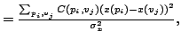
![]() . The edge weight matrix is defined as:
. The edge weight matrix is defined as:
Expanding the numerator of (4) we get ![]() ,
where
,
where
![]() is a
diagonal matrix with
is a
diagonal matrix with
![]() . Using the fact that
. Using the fact that
| (5) |
Putting all these together, we can rewrite (4) as
| (6) |
![\includegraphics[width=0.23 \textwidth, height=0.16 \textwidth]{email/unsortspring.eps}](img60.png)
![\includegraphics[width=0.23 \textwidth, height=0.16 \textwidth]{email/sortspring.eps}](img61.png)